Why practical, again?

In the previous article I shared my approach to engagement with life. The title contains practical to emphasize my approach - it's fulfilling to learn or do something, solving a real problem rather than artificial. Imagine you want to start jogging - until you put your sneakers on and start moving you are not jogging. You can have goals, desires, expectations about jogging, you can learn theory behind it and watch videos but all of this is not the same as jogging. You could gain lots of knowledge but when you practice this knowledge is mostly your narrow representations.

That was a big lesson for me - to engage with the thing I want to do directly. I can give the same example about Deep Learning - I could go through all popular and interesting courses, solve all Kaggle's knowledge or kudos competitions, do homework. All of this doesn't really matter to me because real world - paid competitions and project - have real problems and constraints. They engage you and open for you what you really will be dealing with - creating awesome communications and relationships with clients, handling failures and mistakes, listening to feedback, making your shortcomings visible, marketing yourself. Many things you wouldn't know about.

My Ink

I am writing in a Jupyter notebook which I'll post through fastpages. I'm adding these lines the latest and I give no excuse for inconsistencies. I want you to know that after wrapping the whole thing up I realized that I enjoy writing stories like the previous one more than explaining technical stuff. Partly because it's already explained by someone much better. Partly because I am not interested in this - I am interested in sharing my experience but THE CODE is mostly dry facts.

About the notebook itself, the whole time it feels like I'm trying to fit something here which doesn't fit. Maybe I am not doing it in the right way. Maybe there's no right way. Also it requires some technical preparation, which creates contrast with using medium.com directly - a couple of paragraphs, a proofread and you're done.

The Competition

Let's jump in one of the most practical things for Deep Learning - paid Kaggle competitions. I'll share my solution to Plant Pathology 2020 - FGVC7 which put me in top 23%.

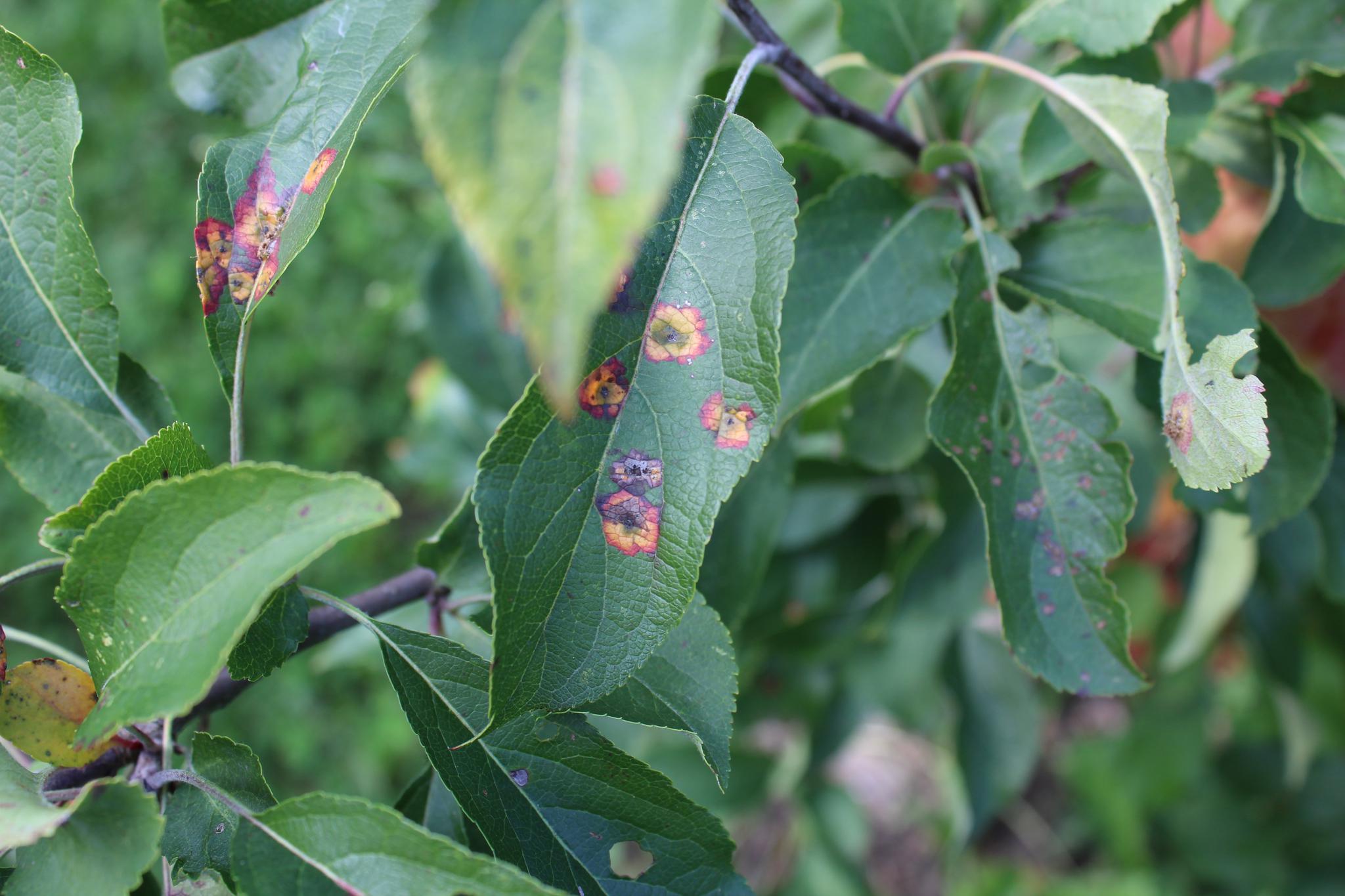
The goal is to build a model which predicts if tree leaves are healthy, have scab, rust or a combination. It made me wonder why so few classes - I'm sure there are much more diseases than just 2. For a given photo like this we have to predict one label: rust

My Approach

I always like to start with something really simple, make it public and build up from it. So first I wrote this notebook which was the base.

I often check other works to see if there's something I don't know, especially the ones with fastai. If I use something in mine I tend to put the source url here on the top. It's my gratitude. Many people optimize for upvoting their work which seems about ego to me. I don't want to please their ego or mine, I want to be authentic and helpful.

#hide_output
!pip install -q git+https://github.com/fastai/fastai2
!pip install -q git+https://github.com/fastai/fastcore
!pip install -q iterative-stratification

I ran this notebook in Colab Pro because it took around 10 hours with 16GB GPU - the Kaggle competition run is limited to 6 hours.

I have a paid plan for Google Drive where I store the data - which actually allowed me to process 500GB and train the model for DeepFake challenge. The cons are that when the number of files gets bigger (350k) drive mounting stops to work. But here it was just 3642 images.

Colab Pro is cheap and easy-to-use.

from google.colab import drive
drive.mount('/content/gdrive', force_remount=True)
!mkdir /root/.kaggle
# imports and folders

from fastai2.vision.all import *
from iterstrat.ml_stratifiers import MultilabelStratifiedKFold

root_dir = Path("/content/gdrive/My Drive/")
path = root_dir/"kaggle/Plants/"
path.mkdir(parents=True, exist_ok=True)
# downloading data from kaggle
# !cp "{root_dir}/kaggle/kaggle.json" /root/.kaggle/kaggle.json
# import kaggle
# !kaggle competitions download -c  plant-pathology-2020-fgvc7 -p "{path}/data" -q
# !unzip -q '{path}/plant-pathology-2020-fgvc7.zip' -d '{path}'
len((path/"images").ls())
3642

The labels are stored in a CSV file and for some reason hot-encoded. Which misrepresents the problem. I think most people who read the description the first time thought it's a multi-label problem (where you need to predict multiple labels for a photo).

train_df = pd.read_csv(path/"train.csv")
train_df.head()
image_id healthy multiple_diseases rust scab
0 Train_0 0 0 0 1
1 Train_1 0 1 0 0
2 Train_2 1 0 0 0
3 Train_3 0 0 1 0
4 Train_4 1 0 0 0

Preparation for k-folds )

It's the first competition where I used cross-validation. It's important to make a right train, valid and test split. The model trains on data from the train split and it validates - calculates the loss and prints metrics - on the valid split. Metrics show us how good is the model.

But test split is something the model only makes predictions on. Kaggle competitions always have the test split prepared - but you don't see its labels, only a public score after submission and a private one after a challenge ends. In fact the private score is calculated on the test set you never see, the reason is to penalize overfitting. On real projects like Canadian housing price prediction I do the splits myself, and I have the labels.

Cross-validation, how I see it, is the idea of minimizing randomness from one split by makings n folds, each fold containing train and validation splits. You train the model on each fold, so you have n models. Then you take average predictions from all models, which supposedly give us more confidence in results.

In my opinion it's more important to make one right split, especially because CV takes n times more to train. But on Kaggle CV yields slightly better scores, thus the environment encourages people to use it. More info about splits and CV you can read in How (and why) to create a good validation set

strat_kfold = MultilabelStratifiedKFold(n_splits=5, random_state=42, shuffle=True)
train_df['fold'] = -1
for i, (_, test_index) in enumerate(strat_kfold.split(train_df.image_id.values, train_df.iloc[:,1:].values)):
    train_df.iloc[test_index, -1] = i
train_df.head()
image_id healthy multiple_diseases rust scab fold
0 Train_0 0 0 0 1 3
1 Train_1 0 1 0 0 0
2 Train_2 1 0 0 0 0
3 Train_3 0 0 1 0 3
4 Train_4 1 0 0 0 2

5 folds, 350 images per each.

train_df.fold.value_counts().plot.bar();
train_df.query("image_id == 'Train_5'")
image_id healthy multiple_diseases rust scab fold
5 Train_5 1 0 0 0 1
get_image_files(path/"images")[5]
Path('/content/gdrive/My Drive/kaggle/Plants/images/Test_64.jpg')

Because there's only one label per row, I transform the dataframe from one-hot to normal label name.

train_df.iloc[0, 1:][train_df.iloc[0, 1:] == 1].index[0]
'scab'

Datablock

# I keep the labels here because I can forget the order. Fuckin up the order fucks up your results.
# LABEL_COLS = ['healthy', 'multiple_diseases', 'rust', 'scab']

The batch size. The batch size affects GPU memory usage. The bigger it is - the faster training. I found the one which uses all the memory.

# BS = 100
BS = 8

That's a fastai data block - the thing which helps to load, label, split and transform the data. It can be read as:

I want something for image categorization,

which I read from images folder using names in my dataframe,

label from the same dataframe,

split using the folds I defined earlier,

resize to the size I want,

and use transforms to help model generalize.

def get_data(fold=0, size=224):
    return DataBlock(blocks    = (ImageBlock, CategoryBlock),
                       get_x=ColReader(0, pref=path/"images", suff=".jpg"),
                       get_y=lambda o:o.iloc[1:][o.iloc[1:] == 1].index[0],
                       splitter=IndexSplitter(train_df[train_df.fold == fold].index),
                       item_tfms=Resize(size),
                       batch_tfms=aug_transforms(flip_vert=True),
                      ).dataloaders(train_df, bs=BS)
dls = get_data()

A batch is a pack of data in GPU memory on which the computations are being done at once. As the size is 8, it means 8 photos are in memory at once. Here they are, with labels. The data is ready.

# dls = dblock.dataloaders(train_df, bs=BS)
dls.show_batch()

Model

Each Kaggle challenge has its own evaluation metric. Here it's ROC AUC which have a scary name - receiver operating characteristic curve. Making things simple is a virtue and a very rare trait in science generally and in AI in particular.

I have no idea why this metric. I won't explain what it means, I think this guy did a really good job. For me it looks like a metric to account for all these TP, FP, TN, FN predictions. I am not going to explain those either.

from sklearn.metrics import roc_auc_score

def roc_auc(preds, targs, labels=range(4)):
    # One-hot encode targets
    targs = np.eye(4)[targs]
    return np.mean([roc_auc_score(targs[:,i], preds[:,i]) for i in labels])

def healthy_roc_auc(*args):
    return roc_auc(*args, labels=[0])

def multiple_diseases_roc_auc(*args):
    return roc_auc(*args, labels=[1])

def rust_roc_auc(*args):
    return roc_auc(*args, labels=[2])

def scab_roc_auc(*args):
    return roc_auc(*args, labels=[3])

Commented code - my experiments. Fastai has lots of state-of-the-art pieces, I tried them one at a time on a smaller dataset and checked if it helped to train a better model.

CutMix is a technique to mix two photos - cut out a piece from one and put it on another. With this we create more combinations, i.e. create new data programmatically without actually taking photos. We make data plenty.

# from fastai2.callback.cutmix import CutMix

And here I tried a weighted loss - a loss that penalizes underrepresented class. Simply put, the number of labels is uneven - we have much fewer photos with multiple disease. When the model calculates loss it just takes the average loss, so we can have a situation where the performance is wonderful on all labels but terrible on multiple diseases. Something everybody wants to be aware of. With weighted loss we pretend this particular class is more important than others by multiplying its loss, so the model tries to optimize it more diligently.

The practice proved that creating multiple metrics and stopping training based on them works here better.

# loss = partial(CrossEntropyLossFlat, weights=tensor([1,1.5,1,1]))

That's all model code and you can compare it with pure Pytorch and TensorFlow2 implementations. Man, these people love to code.

But I simply get the data from a particular fold, create a model, add metrics. I believe resnet152 is the biggest resnet in pytorch. The larger the model - the larger is the capacity to learn differences we want. I also tried the biggest efficientnet just because I saw it somewhere but the best results I had with this

metric = partial(AccumMetric, flatten=False)

def get_learner(fold, size=224):
    dls = get_data(fold, size)
    return cnn_learner(dls, resnet152, metrics=[
                        error_rate,
                        metric(healthy_roc_auc),
                        metric(multiple_diseases_roc_auc),
                        metric(rust_roc_auc),
                        metric(scab_roc_auc),
                        metric(roc_auc)],
#                         cbs=MixUp(0.5),
#                         loss=LabelSmoothingCrossEntropy,
                       ).to_fp16()

Many things are written about learning rate. The things which fastai takes care about, so I chose the default one which works in 95% of cases.

lr = 3e-3

And that's the whole training process. I just trained 5 models on each fold and saved predictions for the test set. I also used big picture size - 450x800, which improved my results in comparison with 224x224. Unsurprisingly, larger images - more data to learn from.

The important thing is to find something to do meanwhile and not to fall a victim of checking constantly how it's going.

test_df = pd.read_csv(path/"test.csv")
test_df.head()

all_preds = []

for i in range(5):
    learn = get_learner(i, (450,800))
    learn.fine_tune(30, lr, freeze_epochs=3)
    tst_dl = learn.dls.test_dl(test_df)
    preds, _ = learn.get_preds(dl=tst_dl)
    all_preds.append(preds)
Downloading: "https://download.pytorch.org/models/resnet152-b121ed2d.pth" to /root/.cache/torch/checkpoints/resnet152-b121ed2d.pth

epoch train_loss valid_loss error_rate healthy_roc_auc multiple_diseases_roc_auc rust_roc_auc scab_roc_auc roc_auc time
0 0.985047 0.573000 0.178571 0.930644 0.741811 0.961710 0.965015 0.899795 01:53
1 0.922874 0.444513 0.148352 0.951735 0.693401 0.959526 0.985851 0.897628 01:51
2 0.576424 0.417532 0.148352 0.931499 0.765575 0.980645 0.984908 0.915657 01:51
epoch train_loss valid_loss error_rate healthy_roc_auc multiple_diseases_roc_auc rust_roc_auc scab_roc_auc roc_auc time
0 0.479184 0.211364 0.071429 0.981382 0.846018 0.995514 0.987069 0.952496 02:30
1 0.364475 0.159768 0.057692 0.992635 0.861272 0.994120 0.993363 0.960347 02:30
2 0.441474 0.193968 0.065934 0.971506 0.840559 0.996421 0.983399 0.947971 02:29
3 0.484192 0.213914 0.057692 0.983447 0.859505 0.989684 0.990516 0.955788 02:30
4 0.435131 0.319889 0.104396 0.958189 0.858703 0.986055 0.985080 0.947007 02:29
5 0.473173 0.320298 0.109890 0.968289 0.784682 0.963609 0.988201 0.926195 02:29
6 0.428352 0.210329 0.068681 0.973533 0.765896 0.999966 0.990945 0.932585 02:30
7 0.419788 0.192607 0.057692 0.989213 0.772640 0.993280 0.993500 0.937158 02:29
8 0.398600 0.264293 0.076923 0.994829 0.781952 0.998320 0.993072 0.942043 02:30
9 0.380230 0.348837 0.104396 0.948462 0.823860 0.995901 0.991459 0.939920 02:30
10 0.343187 2.290655 0.255495 0.824759 0.688343 0.986878 0.953216 0.863299 02:29
11 0.449658 0.191574 0.057692 0.994569 0.806358 0.998958 0.993449 0.948334 02:29
12 0.297756 0.156070 0.046703 0.993676 0.890575 0.995363 0.997222 0.969209 02:29
13 0.326626 0.142823 0.046703 0.987743 0.872110 0.999530 0.996639 0.964005 02:29
14 0.297365 0.194005 0.071429 0.995350 0.774486 0.997984 0.993346 0.940292 02:29
15 0.248781 0.169772 0.043956 0.995015 0.857739 0.989785 0.994889 0.959357 02:29
16 0.247716 0.228961 0.049451 0.971227 0.893545 0.990491 0.992831 0.962024 02:29
17 0.266157 0.151486 0.049451 0.989027 0.905427 0.998236 0.995438 0.972032 02:30
18 0.215115 0.177942 0.041209 0.983168 0.901092 0.992876 0.995558 0.968174 02:30
19 0.215040 0.182103 0.043956 0.991072 0.860067 0.992809 0.994238 0.959547 02:29
20 0.146640 0.174891 0.049451 0.992412 0.899486 0.998068 0.996501 0.971617 02:29
21 0.122240 0.128659 0.041209 0.996057 0.903259 0.999194 0.996056 0.973641 02:29
22 0.164528 0.137511 0.041209 0.996838 0.896757 0.998622 0.995558 0.971944 02:29
23 0.109774 0.137706 0.038462 0.996727 0.912653 0.997597 0.995953 0.975732 02:30
24 0.075488 0.131830 0.043956 0.997266 0.910806 0.997463 0.995781 0.975329 02:30
25 0.054209 0.131286 0.032967 0.996652 0.901252 0.999429 0.995918 0.973313 02:29
26 0.080165 0.154437 0.032967 0.996243 0.911850 0.999530 0.995061 0.975671 02:30
27 0.076159 0.123366 0.035714 0.996336 0.914660 0.999462 0.995575 0.976508 02:29
28 0.067658 0.117424 0.030220 0.997024 0.925658 0.999496 0.995678 0.979464 02:29
29 0.066569 0.127026 0.027473 0.997117 0.913295 0.999630 0.995953 0.976499 02:30
epoch train_loss valid_loss error_rate healthy_roc_auc multiple_diseases_roc_auc rust_roc_auc scab_roc_auc roc_auc time
0 1.214621 0.505084 0.167582 0.954897 0.749839 0.965003 0.946270 0.904002 01:50
1 0.787702 0.411061 0.153846 0.961835 0.699823 0.988642 0.952512 0.900703 01:51
2 0.622221 0.400248 0.109890 0.974966 0.703195 0.991532 0.965906 0.908900 01:51
epoch train_loss valid_loss error_rate healthy_roc_auc multiple_diseases_roc_auc rust_roc_auc scab_roc_auc roc_auc time
0 0.492333 0.300082 0.082418 0.971599 0.795681 0.995968 0.980141 0.935847 02:29
1 0.494743 0.261647 0.071429 0.970427 0.855893 0.998572 0.988870 0.953440 02:29
2 0.359060 0.271687 0.085165 0.979132 0.775450 0.994321 0.990928 0.934958 02:29
3 0.352196 0.229350 0.063187 0.989324 0.790061 0.996774 0.989179 0.941334 02:29
4 0.427697 0.300537 0.118132 0.990310 0.744059 0.997950 0.941691 0.918503 02:29
5 0.513599 0.295712 0.082418 0.983707 0.744701 0.995313 0.946922 0.917661 02:29
6 0.441625 0.358104 0.076923 0.988543 0.716121 0.987147 0.943509 0.908830 02:29
7 0.420680 0.285672 0.071429 0.993806 0.656712 0.992960 0.980312 0.905948 02:30
8 0.426104 0.248101 0.068681 0.990310 0.768465 0.995968 0.974824 0.932392 02:29
9 0.448807 0.259199 0.082418 0.982554 0.772399 0.993313 0.987138 0.933851 02:29
10 0.439116 0.269987 0.063187 0.988766 0.856134 0.993565 0.982096 0.955140 02:29
11 0.397739 0.639953 0.186813 0.979225 0.722704 0.988441 0.979901 0.917568 02:29
12 0.336809 0.223497 0.052198 0.985567 0.826911 0.996774 0.987858 0.949278 02:29
13 0.269442 0.204151 0.071429 0.991612 0.775369 0.999059 0.993655 0.939924 02:29
14 0.241459 0.241700 0.063187 0.987836 0.813985 0.997312 0.982765 0.945474 02:30
15 0.273461 0.207064 0.054945 0.991240 0.809730 0.996405 0.984342 0.945429 02:30
16 0.225611 0.246702 0.065934 0.987092 0.802344 0.998774 0.986606 0.943704 02:29
17 0.205026 0.258343 0.068681 0.986609 0.913455 0.998219 0.987395 0.971420 02:29
18 0.219893 0.201883 0.063187 0.980471 0.857579 0.998017 0.991048 0.956779 02:29
19 0.187929 0.195035 0.049451 0.976918 0.845857 0.998387 0.991922 0.953271 02:29
20 0.125082 0.188541 0.049451 0.994792 0.864001 0.997631 0.993260 0.962421 02:30
21 0.122488 0.201266 0.052198 0.993081 0.864804 0.999194 0.989727 0.961702 02:29
22 0.146725 0.211874 0.063187 0.991742 0.897881 0.998185 0.989230 0.969259 02:30
23 0.115990 0.165340 0.046703 0.994420 0.889130 0.998589 0.993226 0.968841 02:30
24 0.088349 0.175865 0.057692 0.992449 0.913215 0.999362 0.992917 0.974486 02:30
25 0.100924 0.178448 0.057692 0.992002 0.923571 0.999093 0.991288 0.976489 02:30
26 0.092022 0.184467 0.057692 0.991723 0.929271 0.999160 0.992934 0.978272 02:31
27 0.089145 0.188324 0.063187 0.992058 0.929351 0.999160 0.993517 0.978522 02:31
28 0.065488 0.189218 0.060440 0.991891 0.932402 0.998992 0.991528 0.978703 02:30
29 0.099245 0.177854 0.063187 0.990961 0.939146 0.999328 0.993174 0.980652 02:30
epoch train_loss valid_loss error_rate healthy_roc_auc multiple_diseases_roc_auc rust_roc_auc scab_roc_auc roc_auc time
0 1.060653 0.518116 0.175824 0.925740 0.693802 0.947597 0.963552 0.882673 01:50
1 0.796903 0.333589 0.107143 0.976202 0.689146 0.980948 0.981638 0.906983 01:51
2 0.627052 0.355948 0.115385 0.974852 0.784762 0.981317 0.972216 0.928287 01:51
epoch train_loss valid_loss error_rate healthy_roc_auc multiple_diseases_roc_auc rust_roc_auc scab_roc_auc roc_auc time
0 0.465921 0.211115 0.076923 0.990680 0.857097 0.993548 0.984394 0.956430 02:29
1 0.396357 0.230596 0.079670 0.994453 0.823378 0.988172 0.984119 0.947530 02:30
2 0.425156 0.252997 0.101648 0.989423 0.854367 0.989012 0.983774 0.954144 02:30
3 0.394257 0.295605 0.098901 0.986335 0.850353 0.986878 0.980881 0.951112 02:30
4 0.460638 0.353166 0.120879 0.976794 0.646114 0.990323 0.983774 0.899251 02:31
5 0.472251 0.378407 0.112637 0.950906 0.758510 0.985904 0.983636 0.919739 02:31
6 0.449308 0.332915 0.126374 0.980344 0.831005 0.991717 0.983292 0.946590 02:31
7 0.422837 0.316060 0.087912 0.977053 0.691715 0.990894 0.980881 0.910135 02:31
8 0.377337 0.296126 0.076923 0.985762 0.734265 0.988575 0.967686 0.919072 02:31
9 0.417884 0.321095 0.085165 0.975148 0.713953 0.989483 0.988959 0.916886 02:30
10 0.474570 0.321715 0.093407 0.980288 0.542871 0.986190 0.989183 0.874633 02:31
11 0.345946 0.265920 0.096154 0.981657 0.833574 0.989012 0.988649 0.948223 02:30
12 0.334201 0.243763 0.093407 0.971967 0.810854 0.991095 0.985118 0.939759 02:30
13 0.287962 0.302985 0.098901 0.991143 0.796724 0.987685 0.970821 0.936593 02:31
14 0.247122 0.213842 0.063187 0.997596 0.919557 0.988945 0.984946 0.972761 02:31
15 0.266893 0.221402 0.071429 0.987149 0.802344 0.993750 0.991267 0.943627 02:31
16 0.324185 0.199294 0.054945 0.988332 0.756423 0.994892 0.990044 0.932423 02:31
17 0.231756 0.228217 0.065934 0.967308 0.859345 0.970060 0.991405 0.947029 02:30
18 0.214556 0.163841 0.052198 0.992936 0.853645 0.995128 0.985290 0.956750 02:30
19 0.186562 0.240641 0.060440 0.987093 0.908237 0.993280 0.989493 0.969526 02:30
20 0.164244 0.141097 0.038462 0.997596 0.896355 0.995027 0.989080 0.969514 02:29
21 0.209134 0.174100 0.049451 0.994009 0.877168 0.995060 0.991181 0.964354 02:29
22 0.077871 0.146376 0.041209 0.995340 0.901172 0.995363 0.991784 0.970915 02:29
23 0.086250 0.174296 0.049451 0.996191 0.881342 0.988206 0.992731 0.964617 02:29
24 0.065425 0.173790 0.035714 0.996080 0.899566 0.995598 0.991577 0.970705 02:29
25 0.073249 0.161861 0.043956 0.997670 0.909441 0.995010 0.991870 0.973498 02:29
26 0.065725 0.187036 0.041209 0.999223 0.877810 0.995296 0.983792 0.964030 02:28
27 0.119358 0.174043 0.035714 0.998262 0.874117 0.995296 0.991663 0.964834 02:29
28 0.075629 0.172276 0.038462 0.998373 0.878613 0.995296 0.991112 0.965848 02:29
29 0.068883 0.175685 0.038462 0.996117 0.877649 0.995161 0.989458 0.964596 02:30
epoch train_loss valid_loss error_rate healthy_roc_auc multiple_diseases_roc_auc rust_roc_auc scab_roc_auc roc_auc time
0 0.929001 0.764592 0.219780 0.911096 0.816857 0.955679 0.952684 0.909079 01:52
1 0.675620 0.507273 0.164835 0.966019 0.781617 0.979435 0.966016 0.923272 01:53
2 0.617706 0.390988 0.134615 0.934792 0.781236 0.989247 0.968978 0.918563 01:52
epoch train_loss valid_loss error_rate healthy_roc_auc multiple_diseases_roc_auc rust_roc_auc scab_roc_auc roc_auc time
0 0.574120 0.203651 0.071429 0.945133 0.846453 0.993162 0.991629 0.944094 02:30
1 0.301114 0.163122 0.060440 0.988357 0.845309 0.991095 0.997623 0.955596 02:30
2 0.347394 0.214750 0.071429 0.959770 0.853242 0.997077 0.981346 0.947859 02:31
3 0.395934 0.244763 0.076923 0.961611 0.868497 0.998185 0.993868 0.955541 02:30
4 0.450888 0.373079 0.131868 0.763382 0.797712 0.993784 0.979985 0.883716 02:31
5 0.374276 0.607480 0.173077 0.926868 0.850877 0.997480 0.959935 0.933790 02:31
6 0.480051 0.257368 0.085165 0.993788 0.838444 0.990944 0.956404 0.944895 02:31
7 0.508607 0.335371 0.118132 0.981680 0.614569 0.998555 0.981535 0.894085 02:31
8 0.447099 0.305612 0.085165 0.851709 0.834325 0.995867 0.983292 0.916298 02:30
9 0.477192 0.192532 0.054945 0.972882 0.887338 0.996136 0.991543 0.961975 02:30
10 0.368221 0.205813 0.071429 0.989808 0.885126 0.990440 0.993455 0.964707 02:30
11 0.390661 0.266245 0.093407 0.985939 0.819298 0.991465 0.993989 0.947673 02:30
12 0.376762 0.211175 0.054945 0.990738 0.858581 0.991297 0.985204 0.956455 02:31
13 0.295684 0.172537 0.057692 0.994048 0.895271 0.995060 0.991043 0.968856 02:31
14 0.306674 0.681343 0.112637 0.890079 0.941876 0.974143 0.959246 0.941336 02:30
15 0.249741 0.179295 0.057692 0.995908 0.785660 0.998118 0.994144 0.943457 02:30
16 0.280685 0.317672 0.104396 0.960849 0.860870 0.998370 0.992111 0.953050 02:30
17 0.288902 0.178235 0.052198 0.974110 0.898398 0.999462 0.994678 0.966662 02:30
18 0.221528 0.139353 0.052198 0.984544 0.936995 0.999059 0.996521 0.979280 02:30
19 0.175251 0.171660 0.063187 0.996578 0.848360 0.998152 0.993937 0.959257 02:31
20 0.144057 0.206294 0.074176 0.984786 0.910145 0.999110 0.997485 0.972881 02:30
21 0.158589 0.101729 0.027473 0.995090 0.907857 0.999160 0.997020 0.974782 02:31
22 0.140909 0.119903 0.038462 0.982870 0.922502 0.999194 0.997296 0.975465 02:30
23 0.106389 0.158214 0.057692 0.989547 0.884668 0.998370 0.995091 0.966919 02:30
24 0.085377 0.125402 0.043956 0.991296 0.906636 0.999126 0.996314 0.973343 02:31
25 0.062594 0.134993 0.041209 0.988952 0.902975 0.999294 0.996693 0.971979 02:30
26 0.080266 0.146317 0.052198 0.991258 0.894889 0.998891 0.995384 0.970106 02:30
27 0.072346 0.142403 0.049451 0.990998 0.884668 0.998925 0.996142 0.967683 02:30
28 0.084044 0.135851 0.046703 0.991482 0.889550 0.999143 0.996417 0.969148 02:31
29 0.099793 0.128977 0.043956 0.990589 0.892906 0.999160 0.996348 0.969751 02:30
epoch train_loss valid_loss error_rate healthy_roc_auc multiple_diseases_roc_auc rust_roc_auc scab_roc_auc roc_auc time
0 1.053140 0.585916 0.197260 0.940562 0.699648 0.937687 0.967268 0.886291 01:52
1 0.793173 0.608637 0.158904 0.929297 0.615194 0.972405 0.977647 0.873636 01:52
2 0.643487 0.554444 0.142466 0.962314 0.676033 0.981653 0.943440 0.890860 01:52
epoch train_loss valid_loss error_rate healthy_roc_auc multiple_diseases_roc_auc rust_roc_auc scab_roc_auc roc_auc time
0 0.457574 0.308563 0.079452 0.987308 0.749520 0.980308 0.977733 0.923717 02:30
1 0.361474 0.272916 0.060274 0.993960 0.789625 0.980806 0.996192 0.940146 02:30
2 0.426422 0.238606 0.073973 0.989476 0.763849 0.967424 0.996569 0.929329 02:30
3 0.430744 0.348141 0.087671 0.969781 0.810118 0.981089 0.984869 0.936464 02:30
4 0.390538 0.364473 0.104110 0.966872 0.757445 0.964717 0.988438 0.919368 02:31
5 0.430102 0.369142 0.104110 0.952179 0.790826 0.989656 0.984183 0.929211 02:30
6 0.465827 0.263190 0.057534 0.981472 0.847262 0.984027 0.996843 0.952401 02:30
7 0.383814 0.649946 0.167123 0.904061 0.593660 0.979876 0.987923 0.866380 02:30
8 0.399248 0.224631 0.060274 0.992811 0.700528 0.984858 0.991354 0.917388 02:30
9 0.440334 0.282458 0.076712 0.969595 0.818924 0.989739 0.997530 0.943947 02:30
10 0.382763 0.224619 0.063014 0.986178 0.776657 0.983728 0.995780 0.935586 02:30
11 0.364485 0.237379 0.082192 0.984918 0.809238 0.982633 0.996192 0.943245 02:31
12 0.390297 0.266879 0.090411 0.987327 0.723663 0.986086 0.990513 0.921897 02:30
13 0.354540 0.276568 0.093151 0.944064 0.769292 0.991150 0.997581 0.925522 02:31
14 0.324609 0.274236 0.087671 0.976599 0.635607 0.991532 0.997118 0.900214 02:31
15 0.244771 0.252743 0.068493 0.978730 0.833093 0.993774 0.993378 0.949744 02:30
16 0.274489 0.234305 0.068493 0.990699 0.819244 0.987597 0.996792 0.948583 02:30
17 0.230582 0.222373 0.068493 0.983751 0.786904 0.991333 0.995505 0.939373 02:30
18 0.183788 0.205475 0.054795 0.996961 0.845501 0.989523 0.998250 0.957559 02:30
19 0.189672 0.164159 0.046575 0.983528 0.953570 0.993060 0.999245 0.982351 02:31
20 0.136419 0.164070 0.054795 0.987327 0.893692 0.994056 0.998971 0.968511 02:30
21 0.104387 0.170480 0.057534 0.996739 0.911383 0.993591 0.998971 0.975171 02:30
22 0.127624 0.270216 0.076712 0.986437 0.909702 0.991731 0.998216 0.971522 02:30
23 0.136219 0.175872 0.054795 0.995516 0.906180 0.993143 0.998353 0.973298 02:30
24 0.137894 0.227596 0.065753 0.986678 0.911623 0.992512 0.998490 0.972326 02:30
25 0.076939 0.198406 0.060274 0.992959 0.877442 0.993259 0.998868 0.965632 02:30
26 0.110002 0.199703 0.060274 0.996480 0.903858 0.992993 0.997495 0.972707 02:30
27 0.071977 0.183593 0.054795 0.995850 0.908581 0.993657 0.998250 0.974085 02:29
28 0.091631 0.181283 0.054795 0.995701 0.905379 0.993392 0.998593 0.973266 02:29
29 0.054725 0.204143 0.060274 0.995146 0.913545 0.993193 0.998490 0.975093 02:30

Interpretation

Fastai has this helpful tool to check where the model made the most errors. Again, no surprises here - multiple diseases. I actually used it the first time, perhaps mostly for demonstration purposes.

interp = ClassificationInterpretation.from_learner(learn)
interp.plot_top_losses(9, figsize=(15, 10))

Submission

Last but not least, we submit our predictions on the test dataset to Kaggle. We take the average from all 5 models.

subm = pd.read_csv(path/"sample_submission.csv")
preds = np.mean(np.stack(all_preds), axis=0)
subm.iloc[:, 1:] = preds
subm.to_csv("submission.csv", index=False)
pd.read_csv("submission.csv")
image_id healthy multiple_diseases rust scab
0 Test_0 0.006065 0.001795 0.991837 0.000302
1 Test_1 0.001254 0.017110 0.981516 0.000121
2 Test_2 0.001195 0.000296 0.000025 0.998483
3 Test_3 0.999953 0.000004 0.000017 0.000026
4 Test_4 0.000332 0.000758 0.998857 0.000053
... ... ... ... ... ...
1816 Test_1816 0.000228 0.002940 0.996564 0.000268
1817 Test_1817 0.012628 0.051876 0.000738 0.934758
1818 Test_1818 0.001643 0.000960 0.997390 0.000008
1819 Test_1819 0.999675 0.000057 0.000059 0.000209
1820 Test_1820 0.000837 0.038257 0.000094 0.960812

1821 rows × 5 columns

!kaggle competitions submit -c plant-pathology-2020-fgvc7 -f submission.csv -m "450x800"

The practicality I like is that it didn't take me much time to get initial results and then I built from that. I also like that fastai took care about most things, which is clearly visible in comparison with other notebooks.

I think being in top 23% is a good result. There were 1317 participants in total, the first place has 0.98445 score. Good scores which are greater 0.9 start from 1000 place and mine is 295 with 0.96892.